Chapter 24 Regression Analysis with Statistical Tests
This chapter introduces how we estimate the probability that the results from our regression model could have occurred by chance.
24.1 The Population Model and Statistical Tests
In the previous chapters we introduced the concepts of population and sample, and we described how to use regression analysis and the least squares method to estimate a regression model. Our goal is to estimate the relationship that exists in the population, which we call the population’s regression model:
\[\begin{equation} Y = a + bX + V \tag{24.1} \end{equation}\]
where \(Y\) and \(X\) are variables, \(a\) and \(b\) are coefficients, and \(V\) is the error term. With sample data we want to estimate the population values for the constant coefficients \(a\) and \(b\) and find values as close as possible to the population values. In this process there is always some uncertainty, regardless of how many observations we have or how high quality our data is.
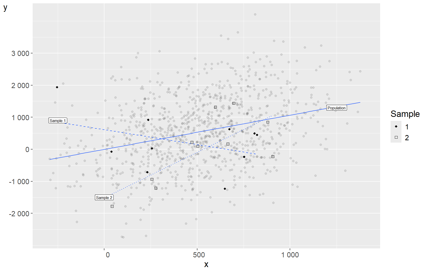
Figure 24.1: Population regression line and two sample regression lines
Description: Figure 24.1 illustrates this with fictitious data. The gray dots are the population in which there exists a positive covariation between the two normally distributed variables \(Y\) and \(X\). The positive covariation is illustrated by the solid line, which is the regression line for the population. From the population of points we have taken two random samples of a few observations and estimated one regression line per sample. Neither of the two samples gives a correct picture of the population’s covariation.
In chapter 19 we introduced statistical tests with null hypothesis and alternative hypothesis. Now we apply these tools to regression coefficients. We start from the population model \(Y = a + bX + V\). For both coefficients \(a\) and \(b\) we set up separate statistical tests and formulate separate null and alternative hypotheses. We are primarily interested in the slope coefficient \(b\) because it describes whether there is a linear covariation between \(X\) and \(Y\). A common way to formulate the null hypothesis for \(b\) is:
\[H_0: b = 0, \qquad H_1: b \neq 0\]
We can also formulate corresponding hypotheses for the intercept: \(H_0: a = 0\) and \(H_1: a \neq 0\). If we estimate \(\hat{b} > 0\) but cannot reject \(H_0: b = 0\) at the chosen significance level \(\alpha\), this indicates that the estimate \(\hat{b} > 0\) could just as well be the result of a random process and we therefore have no reason to assume that \(b \neq 0\).
24.2 Starting Points and Assumptions
Statistical tests for regression coefficients require that certain assumptions hold. These may at first glance seem abstract but will appear more logical as the chapter progresses. They are also discussed more thoroughly in a later chapter. The assumptions are:
Linear model. Our regression model is linear in its coefficients (the coefficients have exponent equal to one) and specified in exactly the way that the relationship between the variables in the population looks.
Random variables. \(Y\) is a random variable from a population with unknown properties. The explanatory variable \(X\) is either from a random sample (observational study) or from a designed process (for example, a controlled experiment). Both \(Y\) and \(X\) are assumed to be random, with each observation \((Y_i, X_i)\) independent and identically distributed (i.i.d.).
Zero conditional mean. The conditional expected value for the error terms is zero: \(E(V \mid X) = 0\). This means that the error terms \(v_i\) do not covary with the explanatory variable \(X\), so \(cov(v, X) = 0\).
Constant variance (homoscedasticity). The error terms have constant variance \(\sigma_V^2\) regardless of which value of \(X\) we compare against: \(var(V \mid X) = \sigma_V^2\), where \(\sigma_V^2 > 0\). This means that along the population regression line, the error terms have the same variance for all values of \(X\).
Uncorrelated errors. The error terms for different observations do not correlate with each other.
Normal errors. The errors of the population model follow a normal distribution, regardless of which values of \(X\) we compare against: \(V \mid X \sim N(0, \sigma_V^2)\).
In this chapter we use these assumptions as theoretical starting points. When we work with real data it is common to encounter situations where one or more assumptions are not fulfilled.
24.3 The Variance of the Regression Model
We described in earlier chapters how to estimate \(\hat{b}\) as:
\[\hat{b} = \frac{\sum_i (x_i - \bar{x})(y_i - \bar{y})}{\sum_i (x_i - \bar{x})^2}\]
The estimated coefficient \(\hat{b}\) is an estimate from a particular sample. The estimator \(\hat{b}\) is a function of the random variables \(x\) and \(y\), so its expected value equals the population value: \(E(\hat{b}) = b\).
Given assumption 6 (that the error terms follow a normal distribution) we assume that the coefficients’ estimators \(\hat{a}\) and \(\hat{b}\) follow a t-distribution. To test \(H_0: b = 0\) vs \(H_1: b \neq 0\) we use a two-sided t-test where the t-value is estimated with:
\[\begin{equation} t = \frac{\hat{b} - b_0}{se(\hat{b})} = \frac{\hat{b}}{se(\hat{b})} \tag{24.2} \end{equation}\]
where \(b_0 = 0\) is the null hypothesis value, and \(se(\hat{b})\) is the standard error of \(\hat{b}\).
To estimate the standard error we take the square root of the variance of the estimator \(\hat{b}\), which is defined as:
\[\begin{equation} var(\hat{b}) = \frac{\sigma_V^2}{\sum_i (x_i - \bar{x})^2} \tag{24.3} \end{equation}\]
The variance of \(\hat{b}\) depends on \(\sigma_V^2\)— the unknown variance of the error terms in the population. Since we cannot observe \(\sigma_V^2\) directly, we estimate it using the mean squared residual (MSR):
\[\begin{equation} \hat{s}_V^2 = \frac{\sum_i (y_i - \hat{y}_i)^2}{n - p} \tag{21.13} \end{equation}\]
where \(p\) is the number of estimated parameters (\(p = 2\) in simple regression: \(\hat{a}\) and \(\hat{b}\)), so the degrees of freedom are \(k = n - p\). Replacing \(\sigma_V^2\) with \(\hat{s}_V^2\) gives the estimated standard error of \(\hat{b}\):
\[\begin{equation} se(\hat{b}) = \sqrt{\frac{\hat{s}_V^2}{\sum_i (x_i - \bar{x})^2}} = \sqrt{\frac{\sum_i (y_i - \hat{y}_i)^2}{(n-p)\,\sum_i (x_i - \bar{x})^2}} \tag{24.4} \end{equation}\]
For the intercept \(\hat{a}\):
\[\begin{equation} var(\hat{a}) = var(\hat{b}) \cdot \frac{\sum_i x_i^2}{n}, \qquad se(\hat{a}) = se(\hat{b}) \cdot \sqrt{\frac{\sum_i x_i^2}{n}} \tag{24.5} \end{equation}\]
24.4 Regression analysis with t-test
Numerical example. Consider a dataset with \(n = 4\) observations: \(x = \{3,\,4,\,6,\,7\}\) and \(y = \{3,\,2,\,5,\,4\}\). The OLS estimates are \(\hat{b} = 0.5\) and \(\hat{a} = 1\), so \(\hat{y} = 1 + 0.5x\).
| \(i\) | \(x_i\) | \(y_i\) | \(\hat{y}_i\) | \(y_i - \hat{y}_i\) | \((y_i - \hat{y}_i)^2\) |
|---|---|---|---|---|---|
| 1 | 3 | 3 | 2.5 | 0.5 | 0.25 |
| 2 | 4 | 2 | 3.0 | \(-1.0\) | 1.00 |
| 3 | 6 | 5 | 4.0 | 1.0 | 1.00 |
| 4 | 7 | 4 | 4.5 | \(-0.5\) | 0.25 |
| Sum | 2.50 |
With \(\bar{x} = 5\) we have \(\sum(x_i - \bar{x})^2 = 4 + 1 + 1 + 4 = 10\). With \(p = 2\) and \(k = n - p = 2\) degrees of freedom:
\[\hat{s}_V^2 = \frac{2.5}{2} = 1.25, \qquad se(\hat{b}) = \sqrt{\frac{1.25}{10}} = \sqrt{0.125} \approx 0.354\]
\[t = \frac{\hat{b}}{se(\hat{b})} = \frac{0.5}{0.354} \approx 1.414\]
The critical value from the t-table with \(k = 2\) degrees of freedom and \(\alpha = 0.05\)(two-sided) is \(t^*_{2,\,0.025} \approx 4.3\). Since \(|t| = 1.414 < 4.3\) we do not reject \(H_0\): the slope is not statistically significantly different from zero at the 5% level.
For the intercept \(\hat{a} = 1\), with \(\sum x_i^2 = 9 + 16 + 36 + 49 = 110\):
\[se(\hat{a}) = 0.354 \cdot \sqrt{\frac{110}{4}} = 0.354 \cdot 5.24 \approx 1.854\]
\[t(\hat{a}) = \frac{1}{1.854} \approx 0.54\]
Again \(|t| < 4.3\), so we do not reject \(H_0: a = 0\) either.
24.5 Regression analysis with confidence interval
A confidence interval for a regression coefficient gives a range of plausible values for the population parameter. For the slope \(b\):
\[\begin{equation} \hat{b} \pm t^*_{k,\,\alpha/2} \cdot se(\hat{b}) \tag{24.6} \end{equation}\]
where \(t^*_{k,\,\alpha/2}\) is the critical value from the t-table with \(k = n - p\) degrees of freedom and significance level \(\alpha/2\) in each tail.
Using the numerical example with \(t^*_{2,\,0.025} = 4.303\):
- CI for \(\hat{b}\): \(0.5 \pm 4.303 \times 0.354 \approx 0.5 \pm 1.52\), giving \((-1.02,\; 2.02)\)
- CI for \(\hat{a}\): \(1 \pm 4.303 \times 1.854 \approx 1 \pm 7.97\), giving \((-6.97,\; 8.97)\)
Both confidence intervals contain zero, which is consistent with not rejecting \(H_0\) at the 5% level. With only \(n = 4\) observations the critical value is large and the intervals are wide. Confidence intervals and hypothesis tests are equivalent: if the CI does not contain the hypothesized value \(b_0\), the test rejects \(H_0\).
24.6 Confidence Interval for the Regression Line
We can also construct a confidence interval for the predicted mean value \(\hat{Y}\) at a specific value \(x_p\). The predicted value is \(\hat{Y}_{x_p} = \hat{a} + \hat{b}\,x_p\), and its standard error is:
\[\begin{equation} se(\hat{Y}_{x_p}) = \sqrt{\hat{s}_V^2 \left(\frac{1}{n} + \frac{(x_p - \bar{x})^2}{\sum_i (x_i - \bar{x})^2}\right)} \tag{24.7} \end{equation}\]
The confidence interval for the mean response at \(x_p\) is \(\hat{Y}_{x_p} \pm t^*_{k,\,\alpha/2} \cdot se(\hat{Y}_{x_p})\).
The standard error in equation (24.7) increases as \(x_p\) moves away from \(\bar{x}\). This means that the CI is narrowest at the mean of \(X\) and widens toward the extremes, producing the characteristic funnel-shaped confidence band shown in figure 24.2.
For the numerical example at \(x_p = 3\):
\[\hat{Y}_3 = 1 + 0.5 \times 3 = 2.5\]
\[se(\hat{Y}_3) = \sqrt{1.25 \left(\frac{1}{4} + \frac{(3-5)^2}{10}\right)} = \sqrt{1.25 \times 0.65} \approx 0.901\]
\[\text{CI: } 2.5 \pm 4.303 \times 0.901 \approx 2.5 \pm 3.88 = (-1.38,\; 6.38)\]
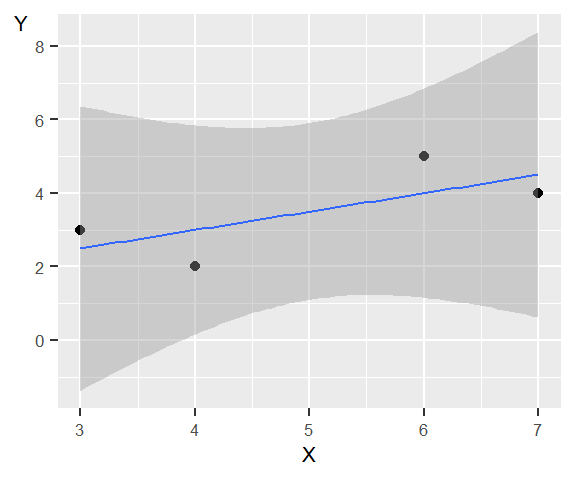
Figure 24.2: Regression line with 95% confidence interval
24.7 Statistical Power in Regression
The precision of our estimates depends on sample size. With a small sample, \(se(\hat{b})\) is large, requiring a large observed effect to reach statistical significance. This leads to low statistical power — the probability of detecting a true effect when it exists.
To illustrate, suppose the true population model is \(Y = 100 + 5X + V\) where \(V \sim N(0, 80)\) and \(X \sim U(0, 1)\). We draw 2,000 samples and estimate the regression model for each, testing \(H_0: b = 0\) at \(\alpha = 0.05\). Figure 24.3 shows the distribution of the 2,000 estimates \(\hat{b}\) for two sample sizes: \(n = 500\) and \(n = 50{,}000\). Black bars show statistically significant results; gray bars show results that are not statistically significantly different from zero.
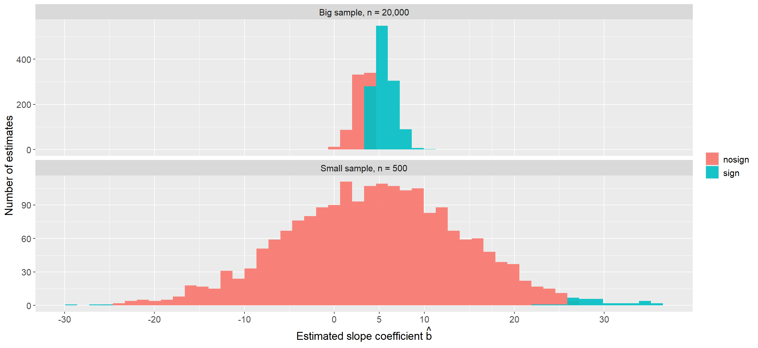
Figure 24.3: Statistical power in regression
In the upper panel (\(n = 500\)) the estimates have a large spread around the true value \(b = 5\) and are mostly not statistically significant. The statistically significant results are concentrated far from the population value — distributed around \(-30\) or \(30\). This is the winner’s curse: when statistical power is low, only extreme estimates can cross the significance threshold, giving a misleading picture of the true effect size.
In the lower panel (\(n = 50{,}000\)) most estimates are statistically significant and all are clearly centered around the population value \(b = 5\).
The more observations we include in our sample, the more accurate the results become, all else equal. By calculating the power of a test we can adjust our analysis to minimize the risk of Type I and Type II errors.
24.8 Statistical and Economic Significance
A statistically significant estimate does not necessarily mean that a result has great importance for the real phenomenon we are studying. Statistical analysis often refers separately to economic significance (sometimes called practical significance) — how much importance our results have in reality. This question generally has no straightforward answer. It depends on the purpose of the study, the type of data, and how the results should be interpreted.
Many people experience, for example, that weather affects their mood. But few would compare normal variations in weather with the effect that earnings or work environment has on their lives. If we succeeded in measuring the causal effect of these phenomena with a regression analysis, the slope coefficient for the weather variable would be relatively small. The slope coefficient for earnings would be larger. Both coefficients could be statistically significantly different from zero. But only one of the variables would have an economically significant effect — that is, have great importance for people’s lives.
Statistical significance depends on the ratio \(\hat{b}/se(\hat{b})\). With a very large sample, even a tiny effect can be statistically significant. A coefficient \(\hat{b} = 0.001\) might be statistically significant at the 1% level while being completely unimportant in practice. Interpreting regression results requires both statistical rigor and subject-matter judgment about what magnitudes matter.
24.9 Chapter Summary
Our goal with regression analysis is to estimate the regression model in a population, the true regression model. With sample data we estimate the model \(Y = a + bX + V\) where \(a\) and \(b\) are coefficients, \(Y\) and \(X\) are variables, and \(V\) is the error term.
Assumptions for regression analysis with the least squares method (do not necessarily need to match real data): (i) the regression model is linear; (ii) \(Y\) is a random variable, \(X\) is either random or from a designed process, observations are i.i.d.; (iii) \(E(V \mid X) = 0\) and \(V\) and \(X\) do not covary; (iv) error terms have constant variance \(var(V \mid X) = \sigma_V^2 > 0\); (v) error terms do not correlate; (vi) \(V \mid X \sim N(0, \sigma_V^2)\).
We estimate \(\hat{a}\) and \(\hat{b}\) and can then perform statistical tests for each coefficient, for example a two-sided t-test with \(H_0: b = 0\), \(H_1: b \neq 0\). For coefficient \(b\) we estimate \(t = (\hat{b} - b_0)/se(\hat{b})\) where \(b_0\) is the null hypothesis value and \(se(\hat{b})\) is the standard error. If the calculated \(|t| > t^*\) given the chosen significance level \(\alpha\), this indicates that \(H_0\) can be rejected as false.
A 95% confidence interval for \(b\) is \(\hat{b} \pm t^*_{k,\,0.025} \cdot se(\hat{b})\). If the CI does not contain zero, the slope is statistically significant.
Note the difference between statistical significance (can we reject \(H_0\) at the chosen significance level?) and economic significance (what importance does the result have for reality?).