Chapter 11 Optimization with functions
This chapter introduces optimization, which we shall use here to find a desired solution based on a function. In social science, we may for example use this to describe how a company can maximize its profit or describe how a person can maximize their utility and happiness or minimize their unhappiness.
11.1 Extreme values
Figure 11.1 shows a line drawn with an unknown function where two points are marked. The lowest point on the line is the function’s minimum value and the highest point is the maximum value. Both of these two are examples of what are called extreme values, also called extreme points or critical points. Consider the following function:
\[ \begin{equation} y=f\left(x\right)=x^{2},\forall1\le x\le10 \end{equation} \]
The symbol \(\forall\) means “for all”. The symbol \(\le\) means “less than or equal to”. The expression \(\forall1\le x\le10\) should be read as “for all \(x\) that are greater than or equal to 1 and less than or equal to 10”. This means that this function is defined over the interval 1 to 10 on the variable \(x\).
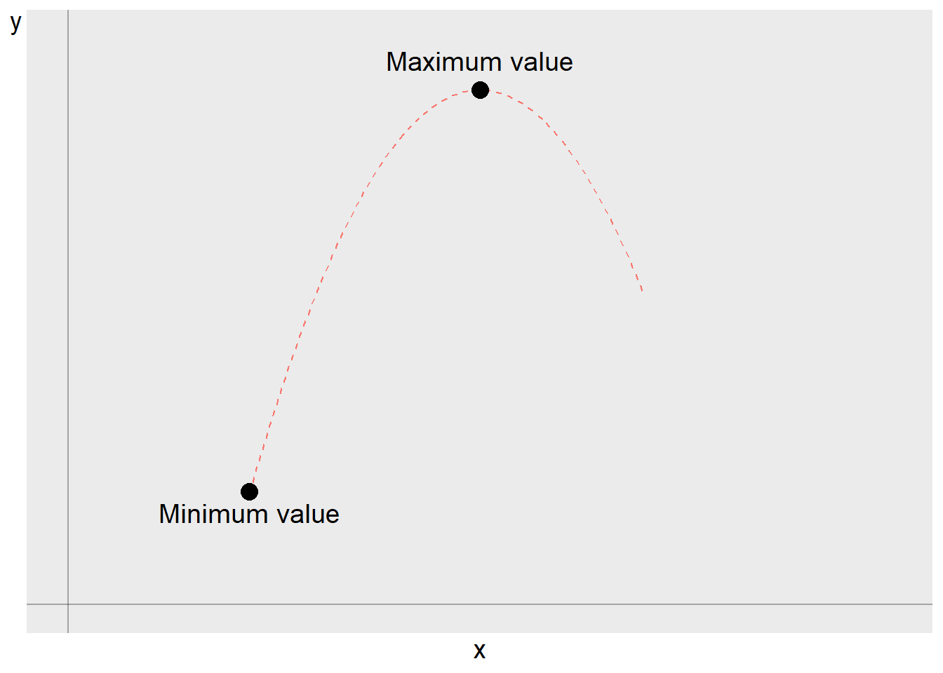
Figure 11.1: A function with a maximum and minimum value
Since \(x\) here can only take a value between 1 and 10, the function \(f\left(x\right)\) and the variable \(y\) will only assume values between \(1^{2}=1\) and \(10^{2}=100\). Our function is relatively simple and we may therefore see that the function’s smallest and largest value in this case are given by these input values:
\[ \begin{align} \text{Smallest value = minimum value: }f\left(1\right) & =1^{2}=1\\ \text{Greatest value = maximum value: }f\left(10\right) & =10^{2}=100\nonumber \end{align} \]
All other values for \(x\) between 1 and 10 result in values for y that are located between these two results. Even a function that is defined over a set can lack extreme values. We can illustrate this with the function:
\[ \begin{equation} y=x,\,\forall x\in\left(0,3\right) \end{equation} \]
In a graph, this function would create a straight line. Since \(x\) is defined over an open interval, the points \(\left(x,y\right)=\left(0,0\right)\) and \(\left(3,3\right)\) are not included. The function is defined infinitely close to the values \(x=0\) and \(x=3\). But for every decimal close to these values, there will be a decimal that is even closer. The function therefore lacks minimum and maximum values.
11.2 Differentiate to find extreme values
The derivative with respect to a variable \(x\) gives us the slope of the line at a specific point. This is a measure of how much the function or the dependent variable, for example \(y\), changes when variable \(x\) increases by 1. We can use this information for different purposes. Suppose we have the following function:
\[ \begin{equation} y=f\left(x\right)=-x^{2},\quad\forall x\in\left[-\infty,\infty\right] \tag{11.1} \end{equation} \]
Function \(f\) describes a desirable phenomenon and we therefore seek the value for \(x\) where \(f\) is maximized. We seek the function’s maximum value, which the derivative can help us with. The function is defined over a bounded interval and is illustrated in figure 11.2 . If the first derivative is equal to 0 at a value on the variable and the line at the point is therefore horizontal and lacks slope, this is an extreme point, minimum or maximum.
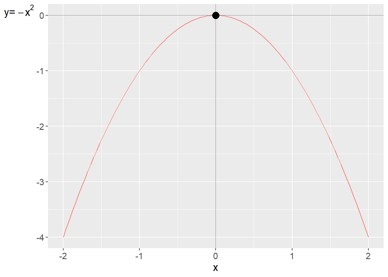
Figure 11.2: The function \(y=f\left(x\right)=x^{2}\)
If we know the function’s second derivative, the slope of the slope, this can also give us more information about what type of extreme point it is. If the second derivative is negative at an extreme point, it means that the points adjacent to the extreme value are smaller than the point and we then know that the extreme value is a maximum point. If the second derivative is positive, the slope of the slope increases, then the extreme value is a minimum point.
To find the function’s extreme points, we calculate the first derivative and set the result equal to 0. This gives us what is called a first-order condition. A first-order condition is a mathematical expression that describes the condition that at the point that is maximum, the first derivative must be equal to 0. From this we can solve for \(x\). From equation (11.1) we get the following first derivative which we set equal to 0:
\[ \begin{align} f'\left(x\right) & =-2x=0 \end{align} \]
This first derivative is equal to 0 at \(x=0\), which is why we from \(f'\left(x\right)=0\) can solve for \(x^{*}=0\). This is the function’s only extreme value. We check the function’s second derivative to see if this is a maximum or minimum point:
\[ \begin{align} f''\left(x\right) & =-2 \end{align} \]
Since the second derivative is negative, \(f''<0\), for all \(x\), \(f\left(x=0\right)\) must be a maximum point. The derivative is not the only way to find a function’s extreme values. Function f is defined for all \(x\in\left[-\infty,\infty\right]\). The function’s minimum is therefore given by the two points \(x=-\infty\) and \(x=\infty\), negative and positive infinity, where the function goes toward negative infinity. Note that this is based on the function being defined for infinity. If the domain instead is \(x\in\left(-\infty,\infty\right)\), where negative and positive infinity are excluded from the domain, then the function lacks a minimum point. There will always be an x-value that results in lower \(f\left(x\right)\). The value \(x=0\) is however still the function’s maximum point. Consider now the following function:
\[ \begin{equation} y=h\left(k\right)=k^{2}-k+3,\quad\forall x\in\left[-\infty,\infty\right] \end{equation} \]
where \(h\) is the name of the function and \(k\) is the variable. To find out for which values of \(k\) the function has its highest and lowest values, we take the first and second derivative:
\[ \begin{align} h'_{k}\left(k\right) & =2k-1\\ h''_{kk}\left(k\right) & =2\nonumber \end{align} \]
From the first derivative we see that \(k^{*}=\frac{1}{2}\). Since the second derivative is \(h''_{kk}>0\), we assume that this is a minimum point. At \(k^{*}=\frac{1}{2}\) we have:
\[ \begin{align} h\left(k^{*}=\frac{1}{2}\right) & =k^{2}-k+3=\left(\frac{1}{2}\right)^{2}-\frac{1}{2}+3=2+\frac{3}{4} \end{align} \]
The function’s line is illustrated in figure 11.3 where the minimum point \(\left(k,y\right)=\left(\frac{1}{2},2.75\right)\) is marked. The function’s maximum is given by the two points \(x=-\infty\) and \(x=\infty\), where function \(h\) goes toward positive infinity.
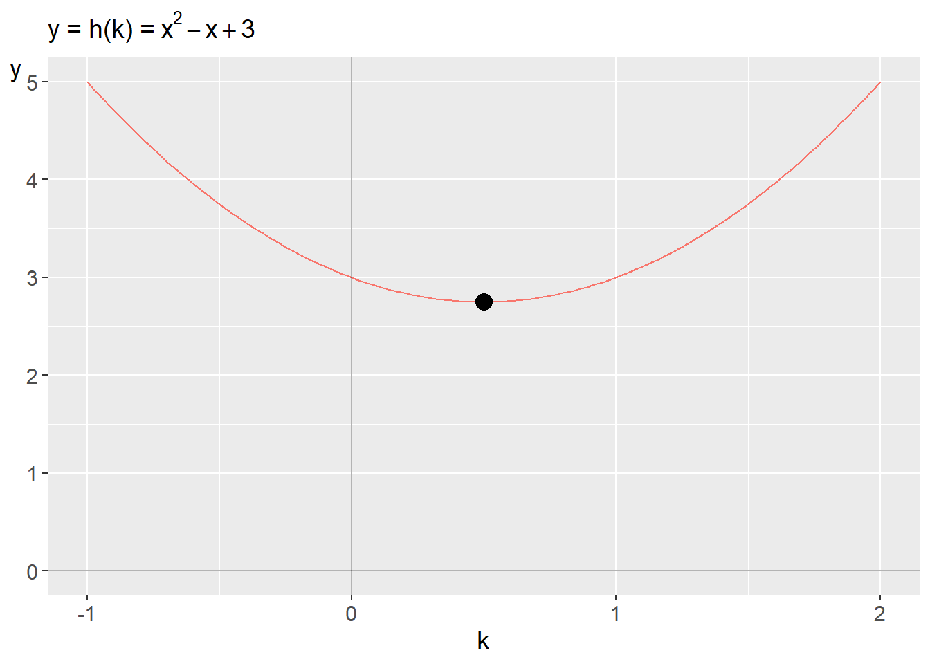
Figure 11.3: The line for \(h\left(k\right)=k^{2}-k+3\) and its minimum point
11.3 Global and local
Maximum and minimum points can be global and local. A local maximum value is the point within an interval where a function assumes its largest value. A global maximum value is the point that gives the function’s largest value over all values that the function is defined for. The same thing for minimum values. Let us illustrate with the following function:
\[ \begin{equation} y=f\left(x\right)=x^{3}-x^{2}-x+2,\quad\forall x\in\left[-10,10\right] \end{equation} \]
This is a third-degree function defined for all \(x\) from \(-10\) to plus 10. The first and second derivatives give:
\[ \begin{align} f'_{x} & =3x^{2}-2x-1\\ f''_{xx} & =6x-2\nonumber \end{align} \]
From the first derivative we solve for two zero points, two values for \(x\) where the first derivative \(f'_{x}\) is equal to 0:
\[ \begin{equation} 3x^{2}-2x-1=0 \end{equation} \]
From the quadratic formula we see that:
\[ \begin{equation} x^{*}=-\left(-\frac{2/3}{2}\right)\pm\sqrt{\left(-\frac{2/3}{2}\right)^{2}-\left(-1/3\right)} \end{equation} \]
This gives the solutions \(x_{1}=-\frac{1}{3}\) and \(x_{2}=1\). At these two points \(f'=0\). We check the solutions by substituting the values into the second derivative:
\[ \begin{align} f''_{xx}\left(-\frac{1}{3}\right) & =6\left(-\frac{1}{3}\right)-2=-4\\ f''_{xx}\left(1\right) & =6*1-2=4\nonumber \end{align} \]
The first row means that the second derivative is negative at \(x=-\frac{1}{3}\). This indicates that this is a maximum point. The second row gives that the second derivative is positive at \(x=1\), which suggests that this is a minimum point. Let us also calculate \(y\) at these points:
\[ \begin{align*} y=f\left(x=-\frac{1}{3}\right) & =x^{3}-x^{2}-x+2\\ & =\left(-\frac{1}{3}\right)^{3}-\left(-\frac{1}{3}\right)^{2}-\left(-\frac{1}{3}\right)+2\\ & =-\frac{1}{27}-\frac{1}{9}+\frac{1}{3}+2\\ & =2+\frac{5}{27} \end{align*} \]
For \(x=1\) we have:
\[ \begin{align} y=f\left(x=1\right) & =x^{3}-x^{2}-x+2=\left(1\right)^{3}-\left(1\right)^{2}-\left(1\right)+2=1 \end{align} \]
The function is defined for all \(x\in\left[-10,10\right]\). Let us also calculate \(y\) for the endpoints (the outer values) \(-10\) and 10. For \(x=-10\):
\[ \begin{align*} y=f\left(x=-10\right) & =x^{3}-x^{2}-x+2\\ & =\left(-10\right)^{3}-\left(-10\right)^{2}-\left(-10\right)+2\\ & =-1,000-100+10+2\\ & =-1,088 \end{align*} \]
For \(x=10\):
\[ \begin{align} y=f\left(x=10\right) & =x^{3}-x^{2}-x+2\\ & =\left(10\right)^{3}-\left(10\right)^{2}-\left(10\right)+2\nonumber \\ & =1,000-100-10+2\nonumber \\ & =892\nonumber \end{align} \]
The function’s value at x=-10 is smaller than the value at \(x=1\), since \(-1,088<1\) and the function’s value at \(x=10\) is larger than at \(x=-\frac{1}{3}\) since \(892>2+\frac{5}{27}\). We therefore conclude that the function’s global minimum is at \(\left(x,y\right)=\left(-10,-1,088\right)\) and its global maximum is at \(\left(x,y\right)=\left(10,892\right)\). Additionally, the function has a local minimum at the point \(\left(x,y\right)=\left(1,1\right)\) and a local maximum at \(\left(x,y\right)=\left(-\frac{1}{3},2+\frac{5}{27}\right)\).
The next question is how local these extreme values are, within which intervals of \(x\) are these points maximum and minimum? We start by looking at this in a graph, which is illustrated in figure 11.4 . The two local extreme values are marked along the line with points. The global extreme values at \(x=-10\) and \(x=10\) are outside the picture and marked with arrows.
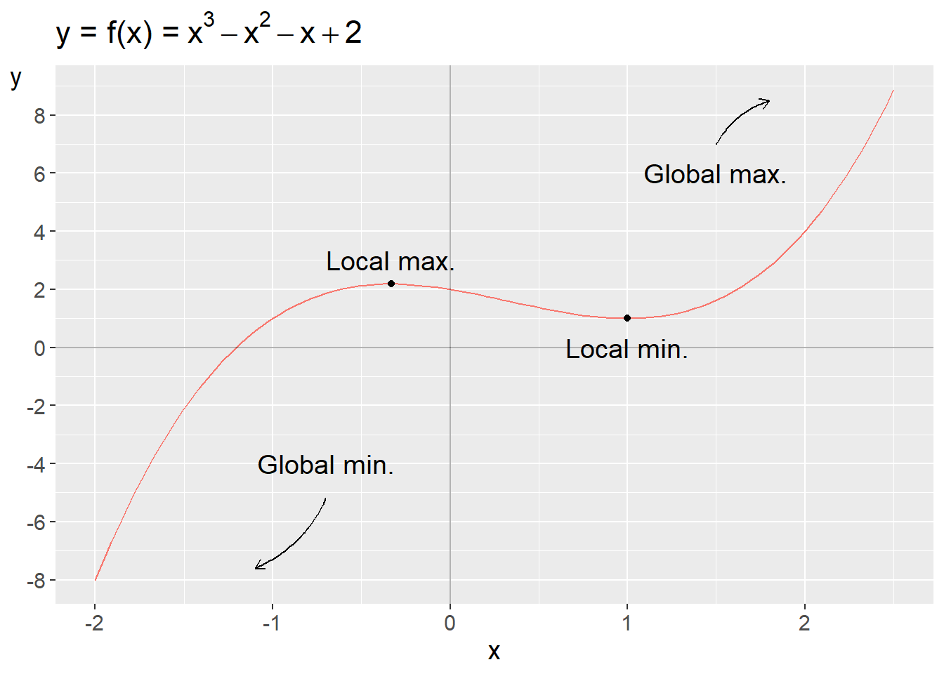
Figure 11.4: Local and global minimum and maximum points
From the picture we see that the point \(\left(x,y\right)=\left(1,1\right)\) is a minimum for the function for \(x\)-values from \(-1\) and upward. For all values for \(x\) above \(-1\) up to 10 (the function’s domain), the point \(\left(1,1\right)\) is the one that gives the lowest value. For the point \(\left(x,y\right)=\left(-\frac{1}{3},2+\frac{5}{27}\right)\) we see that this is the function’s maximum for all \(x\) from approximately 1.6 and downward.
11.4 More examples
Let us find the extreme values for some functions. We seek the largest and smallest value, maximum and minimum value. Let us start with the function:
\[ \begin{equation} y=f\left(x\right)=x,\quad\forall x\leq0 \end{equation} \]
Since \(f\) is defined for \(x\leq0,y=f\left(0\right)=0\) is the function’s largest value, its global maximum value. Since \(f\) is defined for all negative values, y goes toward negative infinity, \(-\infty\), when \(x\) does the same, which is the function’s global minimum value. If we instead have the function:
\[ \begin{equation} y=f\left(x\right)=x,\quad\forall x<0 \end{equation} \]
where the value 0 is excluded from the domain, then the function lacks a global maximum value. We only come infinitely close to 0. The minimum value is also here negative infinity, \(-\infty\). Let us now take the function:
\[ \begin{equation} y=f\left(x\right)=3x,\quad\forall x\in\left(2,12\right) \end{equation} \]
The domain \(\left(2,12\right)\) excludes the values 2 and 12. The function therefore lacks global minimum and maximum values. If the function is instead defined for \(x\in\left[2,12\right]\), the function’s global minimum value is:
\[ \begin{equation} y=f\left(2\right)=6 \end{equation} \]
The function’s global maximum value:
\[ \begin{equation} y=f\left(12\right)=36 \end{equation} \]
Let us now calculate the global minimum and maximum value for the following function:
\[ \begin{equation} y=f\left(x\right)=x^{2}-x,\quad\forall x\in\mathbb{R} \end{equation} \]
We take the first and second derivatives of \(y\) with respect to \(x\):
\[ \begin{align} y'_{x} & =2x-1\\ y''_{xx} & =2\nonumber \end{align} \]
From the first derivative we see that \(x=\frac{1}{2}\). This gives the following value for \(y\):
\[ \begin{equation} y=f\left(\frac{1}{2}\right)=\left(\frac{1}{2}\right)^{2}-\frac{1}{2}=-\frac{1}{4} \end{equation} \]
The second derivative is \(y''_{xx}>0\) which means that this is a global minimum value. Since the function is defined over the real numbers \(\mathbb{R}\), which does not include infinity, the function lacks a global maximum value.
11.5 Terrace
Let us now look at the line in figure 11.5 . At the two marked points in the diagram, the first derivative is equal to 0. In the figure, the point \(\left(x,y\right)=\left(-0.5,-1.7\right)\) is a minimum point. At the point \(\left(1,0\right)\), the second derivative is equal to 0, which is why this is a terrace point. At the terrace point, our function increases for larger values of \(x\) and decreases for smaller values of \(x\). Let us summarize what applies for the second derivative for points where the first derivative is equal to 0. We have the following rules:
\[ \begin{align} \text{Maximimum point: }f'' & <0\\ \text{Minimimum point: }f'' & >0\nonumber \\ \text{Terrace point: }f'' & =0\nonumber \end{align} \]
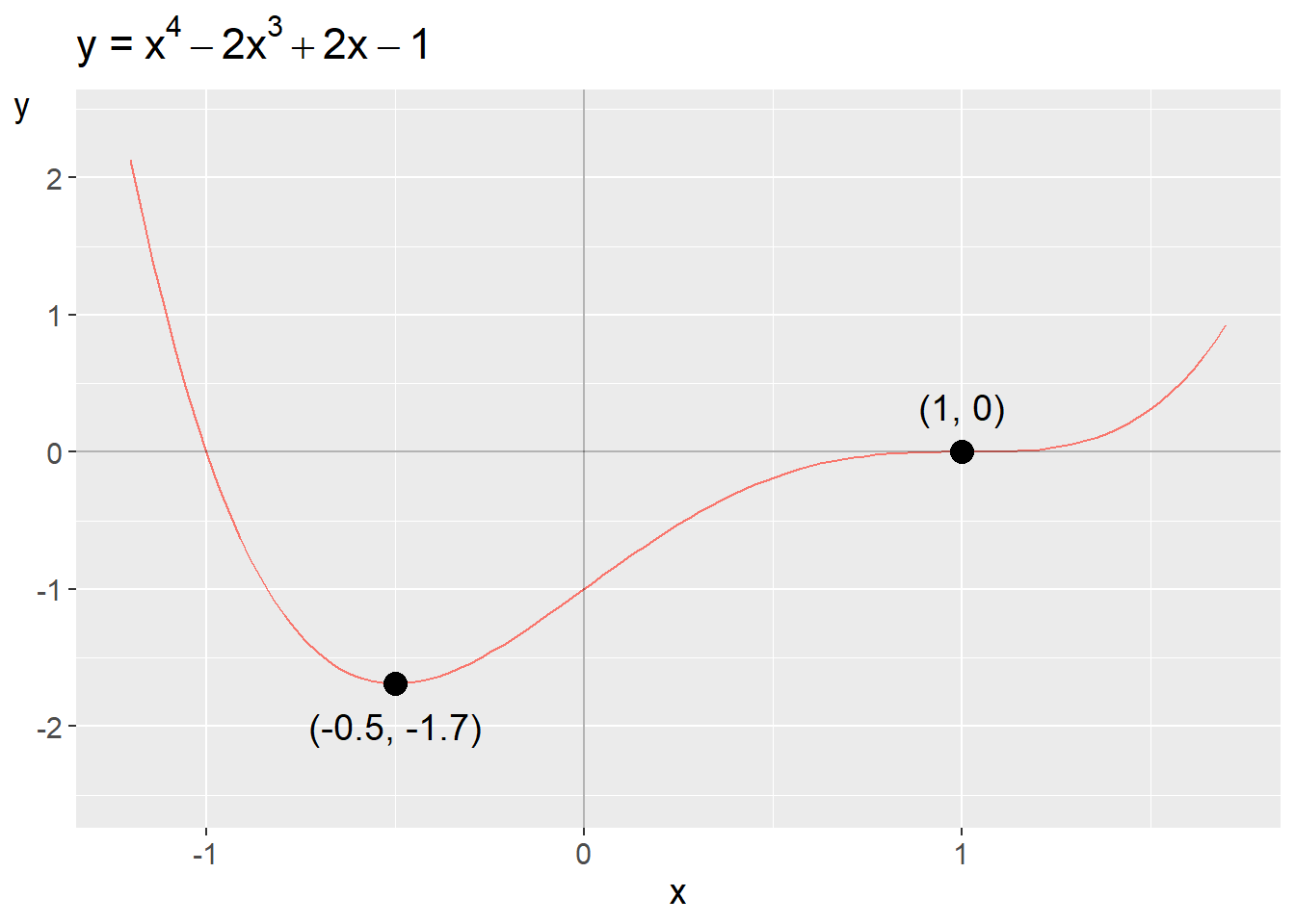
Figure 11.5: Function with minimum and terrace point
The function for the line in figure 11.5 is:
\[ \begin{equation} y=f\left(x\right)=x^{4}-2x^{3}+2x-1 \tag{11.2} \end{equation} \]
The first derivative with respect to \(x\):
\[ \begin{equation} f'_{x}\left(x\right)=4x^{3}-6x^{2}+2 \tag{11.3} \end{equation} \]
The second derivative with respect to \(x\):
\[ \begin{equation} f''_{xx}\left(x\right)=12x^{2}-12x \tag{11.4} \end{equation} \]
Try yourself to find these functions’ solutions.
11.6 Optimization with constraints
So far we have worked with optimization to find extreme values in functions without any particular form of limitation, other than the function itself. Often, however, we have use of being able to add constraints to our calculations. We often have use of this in social science, for example in reasoning about how people and organizations try to achieve their goals based on limited means or opportunities. Constraints can however make it more difficult to find the solution to optimization problems.
A common method for finding extreme points with constraints is the Lagrange method. We begin by describing the method on a brief overall level. Suppose we shall optimize function \(f\left(x\right)\) with respect to a constraint that we formulate generally as function \(g\left(x\right)=0\). We begin by just writing this as a function:
\[ \begin{align} \max_{x}f\left(x\right),\quad\text{w.r.t. }g\left(x\right) & =0 \end{align} \]
Function \(f\) shall be maximized with respect to variable \(x\) so that function g is equal to 0. The abbreviation “w.r.t” stands for with respect to . Sometimes the abbreviation “s.t.” is used which stands for subject to . Then we set up the Lagrange function:
\[ \begin{equation} \mathcal{L}\left(x,\lambda\right)=f\left(x\right)+\lambda g\left(x\right) \tag{11.5} \end{equation} \]
where the Greek letter small lambda \(\lambda\) symbolizes the Lagrange multiplier, which in the Lagrange function is a new variable that is connected with the Lagrange method. We shall return to the interpretation of \(\lambda\). For the functions f and g to be able to be set up in this way, we may need to rewrite them. To find the extreme points, we differentiate the Lagrange function with respect to the two variables x and \(\lambda\):
\[ \begin{align} \mathcal{L}'_{x} & =f'_{x}+\lambda g'_{x}\\ \mathcal{L}'_{\lambda} & =g\nonumber \end{align} \]
If we set these expressions equal to 0, we get the first-order conditions and can solve for any solutions for \(x\) and \(\lambda\). The Lagrange multiplier \(\lambda\) has a specific interpretation depending on the maximization problem itself and can for example indicate changes with respect to if the constraint, which \(\lambda\) is multiplied by, changes by one unit. Let us illustrate by maximizing the following function:
\[ \begin{equation} f\left(x\right)=x^{2} \end{equation} \]
While we maximize \(f\left(x\right)\), we shall fulfill the following constraint: \(x^{2}=2\). We call this expression function \(g\left(x\right)\) and move all terms in the function to one side of the equals sign so that we get \(g\left(x\right)=0\):
\[ \begin{align*} g\left(x\right) & =x^{2}-2=0 \end{align*} \]
Now we set up the Lagrange function in the following way:
\[ \begin{align} \mathcal{L}\left(x,\lambda\right) & =f\left(x\right)+\lambda g\left(x\right)\\ \mathcal{L}\left(x,\lambda\right) & =x^{2}+\lambda\left(x^{2}-2\right)\nonumber \end{align} \]
To find the function’s solutions, we take the derivative of \(\mathcal{L}\) with respect to x and \(\lambda\). By setting these respective derivatives equal to 0, we get the first-order conditions:
\[ \begin{align} \mathcal{L}'_{x} & =2x+2x\lambda=0\\ \mathcal{L}'_{\lambda} & =x^{2}-2=0\nonumber \end{align} \]
From \(\mathcal{L}'_{x}\) we get the solution for \(\lambda\):
\[ \begin{align} \lambda^{*} & =-1 \end{align} \]
From \(\mathcal{L}'_{\lambda}\) we get the solution for \(x\):
\[ \begin{equation} x^{*}=\sqrt{2} \end{equation} \]
This means that if we shall maximize the function \(f\left(x\right)=x^{2}\) so that the constraint \(x^{2}-2=0\) is fulfilled, then \(x^{*}=2^{1/2}\approx1,41\). Let us now take the following maximization problem with constraints:
\[ \begin{align} \text{Maximize }f\left(x,y\right) & =x^{2}y\\ \text{under the condition }g\left(x,y\right) & =x+y=10\nonumber \end{align} \]
We solve this by setting up the Lagrange function:
\[ \begin{equation} \mathcal{L}\left(x,y,\lambda\right)=x^{2}y+\lambda\left(x+y-10\right) \end{equation} \]
From this we derive the partial derivatives and set these equal to 0 to get the first-order conditions:
\[ \begin{align} \mathcal{L}'_{x}: & 2xy+\lambda=0\\ \mathcal{L}'_{y}: & x^{2}+\lambda=0\nonumber \\ \mathcal{L}'_{\lambda}: & x+y-10=0\nonumber \end{align} \]
Since \(\mathcal{L}'_{x}=\mathcal{L}'_{y}=0\), we create respective definitions of \(\lambda\):
\[ \begin{align} \mathcal{L}'_{x}:\lambda & =2xy\\ \mathcal{L}'_{y}:\lambda & =x^{2}\nonumber \end{align} \]
By setting the definitions of \(\lambda\) equal to each other, we get a new constraint:
\[ \begin{align} x^{2} & =2xy \tag{11.6} \end{align} \]
We simplify this by dividing both sides by \(x\):
\[ \begin{align} x & =2y \tag{11.7} \end{align} \]
We also have the constraint left:
\[ \begin{equation} x+y-10=0 \tag{11.8} \end{equation} \]
Based on this we now solve for \(x\) and \(y\). We have \(x=2y\), which we substitute into equation (11.8) :
\[ \begin{align} x+y-10 & =0\\ 2y+y-10 & =0\nonumber \end{align} \]
This gives us the solution \(y^{*}=\frac{10}{3}\). This \(y\) we use in equation (11.7) , \(x=2y\), and solve for \(x\):
\[ \begin{equation} x^{*}=\frac{20}{3} \end{equation} \]
These are the values for x and y that optimize \(f\left(x,y\right)=x^{2}y\), while the constraint \(x+y=10\) is fulfilled:
\[ \begin{align} f\left(x^{*},y^{*}\right) & =f\left(\frac{20}{3},\frac{10}{3}\right)=\left(20/3\right)^{2}\left(10/3\right)=\frac{4,000}{27} \end{align} \]
11.7 Chapter summary
A function can have maximum and minimum points where the function’s value is maximized or minimized. These are called extreme points.
One way to find extreme points is to use derivatives and calculate a line’s slope at a specific point. The first derivative gives the line’s slope, the second derivative gives the slope of the slope, and so on. To calculate the derivative we use limits, limes.
Example: the function \(y=f\left(x\right)=x^{2}\) has first derivative \(f'=2x\) and second derivative \(f''=2\).
If the first derivative is \(f'=0\) at a point, this is a maximum point if \(f''<0\), minimum point if \(f''>0\) and terrace point if \(f''=0\).
The Lagrange method is a method for solving maximization or minimization problems with constraints. The general form for the Lagrange function is \(\mathcal{L}\left(x,\lambda\right)=f\left(x\right)+\lambda g\left(x\right)\) where \(\lambda\) is the Lagrange multiplier and \(g\) is the function for the constraint.