Chapter 10 Derivative
This chapter introduces the derivative. The derivative is a function for calculating the slope of a line at a specific point. The derivative can be used to find a function’s maximum and minimum values, which is central to a large amount of analytical work.
10.1 Limit
Before we get to derivatives, we shall introduce limits. The limit is the value that a function approaches at a specific point. Limits can be used to handle expressions that are not defined for all numbers. Suppose we have the function:
\[ \begin{equation} y=f\left(x\right)=\frac{1}{x^{2}} \end{equation} \]
where \(x\) is a real number. The real numbers are not defined for division by 0. To understand why, see what happens with \(f\left(x\right)\) when \(x\) approaches 0:
\[ \begin{align} \text{For }x=0.1\text{ is }\frac{1}{x^{2}} & =\frac{1}{0.01}=100\\ \text{For }x=0.01\text{ is }\frac{1}{x^{2}} & =\frac{1}{0.0001}=10,000\nonumber \\ \text{For }x=0.0001\text{ is }\frac{1}{x^{2}} & =\frac{1}{0.0000001}=100,000,000\nonumber \tag{10.1} \end{align} \]
When \(x\) approaches 0, the expression \(1/x^{2}\) approaches infinity. Infinity is written with the symbol \(\infty\), which is not a real number. This means that the function \(y=f\left(x\right)=1/x^{2}\) is not defined for \(x=0\). To describe that \(f\left(x\right)\) is defined for all \(x\) except 0 one may write:
\[ \begin{equation} y=f\left(x\right)=\frac{1}{x^{2}},\,\forall x\neq0 \end{equation} \]
The variable \(y\) is a function of \(x\) for all \(x\) that are not equal to 0. That equation (10.1) approaches infinity as \(x\) approaches 0 can be described in the following way:
\[ \begin{equation} \lim_{x\rightarrow0}f\left(x\right)=\frac{1}{x^{2}}=\infty \end{equation} \]
The expression \(\lim_{x\rightarrow0}\) stands for limes, which means limit. To describe how function \(f\) behaves when \(x\) goes toward positive infinity, we write:
\[ \begin{equation} \lim_{x\rightarrow\infty}f\left(x\right)=\frac{1}{x^{2}}=0 \end{equation} \]
When \(x\) goes toward positive infinity, the limit for \(f\left(x\right)=1/x=0\). The function goes toward the value 0. For many expressions, it’s possible to find the limit by calculating the expression for values close to the limit, as in equation (10.1) . Suppose we seek the limit for the expression \(x-1\) when \(x\rightarrow1\):
\[ \begin{equation} \lim_{x\rightarrow1}x-1 \end{equation} \]
To find the limit, we calculate values close to \(x=1\):
| \(x\) | \(x-1\) |
|---|---|
| 0.9 | 0.1 |
| 0.99 | 0.01 |
| 0.999 | 0.001 |
The closer \(x\) gets to 1, the closer \(x-1\) gets to the value 0. This is the limit for \(x-1\):
\[ \begin{equation} \lim_{x\rightarrow1}x-1=0 \end{equation} \]
We also calculate \(x-1\) for values just above 1:
| \(x\) | \(x-1\) |
|---|---|
| 1.1 | 0.1 |
| 1.01 | 0.01 |
| 1.001 | 0.001 |
We get the same limit regardless of whether we approach \(x\) from above or from below. The limit for an expression can however differ depending on whether we approach the limit from above or from below. Take for example the function:
\[ \begin{equation} y=\frac{1}{x}\,\forall x\neq0 \end{equation} \]
The function \(y=\frac{1}{x}\) is defined for all \(x\) that are not equal to 0. For \(x>0\), the same limit still applies as for \(y=f\left(x\right)=1/x^{2}\). When \(x\) approaches 0 from values above 0, the expression \(1/x\) goes toward positive infinity. But if we instead look at how \(x\) approaches 0 for values below 0, we get the following result instead:
\[ \begin{align} \text{For }x=-1\text{ is }y=\frac{1}{x} & =\frac{1}{-1}=-1\\ \text{For }x=-0.2\text{ is }y=\frac{1}{x} & =\frac{1}{-0.2}=-5\nonumber \\ \text{For }x=-0.0001\text{ is }y=\frac{1}{x} & =\frac{1}{-0.0001}=-10,000\nonumber \end{align} \]
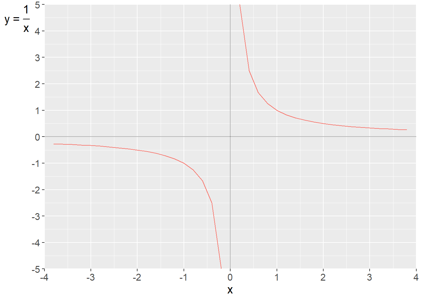
Figure 10.1: The function \(y=f\left(x\right)=1/x\)
Since \(x\) approaches 0 from values below 0, \(1/x\) goes toward negative infinity, which can be written \(-\infty\). This is illustrated in figure 10.1 where function \(f\left(x\right)=1/x\) goes toward positive infinity \(+\infty\) as \(x\) approaches 0 for positive numbers and toward negative infinity \(-\infty\) for negative numbers:
\[ \begin{align} \lim_{x\rightarrow0^{+}} & f\left(x\right)=\frac{1}{x}=+\infty\\ \lim_{x\rightarrow0^{-}} & f\left(x\right)=\frac{1}{x}=-\infty\nonumber \end{align} \]
The notation \(x\rightarrow0^{+}\) means that \(x\) goes toward 0 from the positive side of the input value \(\left(x>0\right)\). This is also called a right-hand limit, because \(x\) approaches from the right on the number line. The expression \(x\rightarrow0^{-}\) means that \(x\) approaches 0 from smaller values \(\left(x<0\right)\), which is called a left-hand limit.
10.2 Simplify first
We often benefit from simplifying the function we are working with as far as possible. This also applies when we seek limits. Consider now the following equation:
\[ \begin{equation} y=g\left(x\right)=\frac{x^{3}-2x^{2}+4x-8}{x-2} \end{equation} \]
If we substitute \(x=2\), we get:
\[ \begin{align} g\left(2\right) & =\frac{2^{3}-2*2^{2}+4*2-8}{2-2}=\frac{0}{0} \end{align} \]
For \(x=2\) the nominator and denominator is zero, which is undefined for real values. It is however possible to calculate the limit as \(x\) approaches 2 and thereby get a value for \(g\left(2\right)\). But first we factorize the numerator so we get:
\[ \begin{align} y=g\left(x\right) & =\frac{x^{3}-3x^{2}+3x-9}{x-2}=\frac{\left(x^{2}+4\right)\left(x-2\right)}{x-2} \end{align} \]
Since we have the parenthesis \(\left(x-2\right)\) in both numerator and denominator, we can cancel this and get:
\[ \begin{align} g\left(x\right) & =\frac{\left(x^{2}+4\right)\cancel{\left(x-2\right)}}{\cancel{\left(x-2\right)}}=x^{2}+4 \end{align} \]
In this simplified form the function is defined for \(x=2\):
\[ \begin{equation} y=g\left(2\right)=2^{2}+4=8 \end{equation} \]
Since this is a simplified version of the function we call this value 8 the function’s limit for \(x=2\), which we write as:
\[ \begin{equation} \lim_{x\rightarrow2}g\left(x\right)=\frac{x^{3}-2x^{2}+4x-8}{x-2}=8 \end{equation} \]
Suppose now that we have the following function:
\[ \begin{align} y=f\left(x\right) & =\frac{\left(x^{2}+3\right)\left(x-3\right)}{x-2} \end{align} \]
for \(x=2\) the denominator is zero and therefore undefined. First we can expand the numerator: \(\left(x^{2}+3\right)\left(x-3\right)=x^{3}-3x^{2}+3x-9\). We cannot simplify the expression more. In this case we have two limits. As \(x\) approaches 2 from the left \(\left(x<2\right)\) the function \(f\left(x\right)\) approaches positive infinity \(+\infty\). As \(x\) approaches 2 from the right \(\left(x>2\right)\) function \(f\left(x\right)\) approaches negative infinity \(-\infty\):
\[ \begin{align} \lim_{x\rightarrow2^{+}}f\left(x\right) & =\frac{x^{3}-3x^{2}+3x-9}{x-2}=-\infty\\ \lim_{x\rightarrow2^{-}}f\left(x\right) & =\frac{x^{3}-3x^{2}+3x-9}{x-2}=+\infty\nonumber \end{align} \]
While limits help us understand function behavior near problematic points, they also enable us to solve a fundamental question: how can we measure the exact slope of a curved line at a single point? This leads us to the derivative.
10.3 Differentiating
The derivative can be used to calculate the slope of a line at a specific point. In section 4.4 we went through the equation of the straight line. In a function of the form \(y=a+bx\), \(b\) is the slope of the line and \(a\) is the value \(y\) takes when \(x=0\). b is a measure of how much \(y\) changes when \(x\) increases by 1. Since the line is straight, it has the same slope regardless of which value \(x\) has. The slope between the points \(\left(x_{1},y_{1}\right)\) and \(\left(x_{2},y_{2}\right)\) we may calculate as:
\[ \begin{equation} b=\frac{y_{2}-y_{1}}{x_{2}-x_{1}} \end{equation} \]
If we instead have a line that is not straight over all values of \(x\), one may use the derivative to calculate the slope at a specific value of \(x\). Let us illustrate with the function
\[ \begin{equation} y=x^{2} \end{equation} \]
Figure 10.2 illustrates how the slope of the line for \(x^{2}\) varies depending on the value for x. The solid curved line is drawn with \(x^{2}\) and the dashed straight lines show the slope at two points on the curved line. At the point \(\left(x,y\right)=\left(0,0\right)\) the solid line has slope 0 and is horizontal. At the point \(\left(x,y\right)=\left(2,4\right)\) the slope is instead positive, up toward the graph’s right corner.
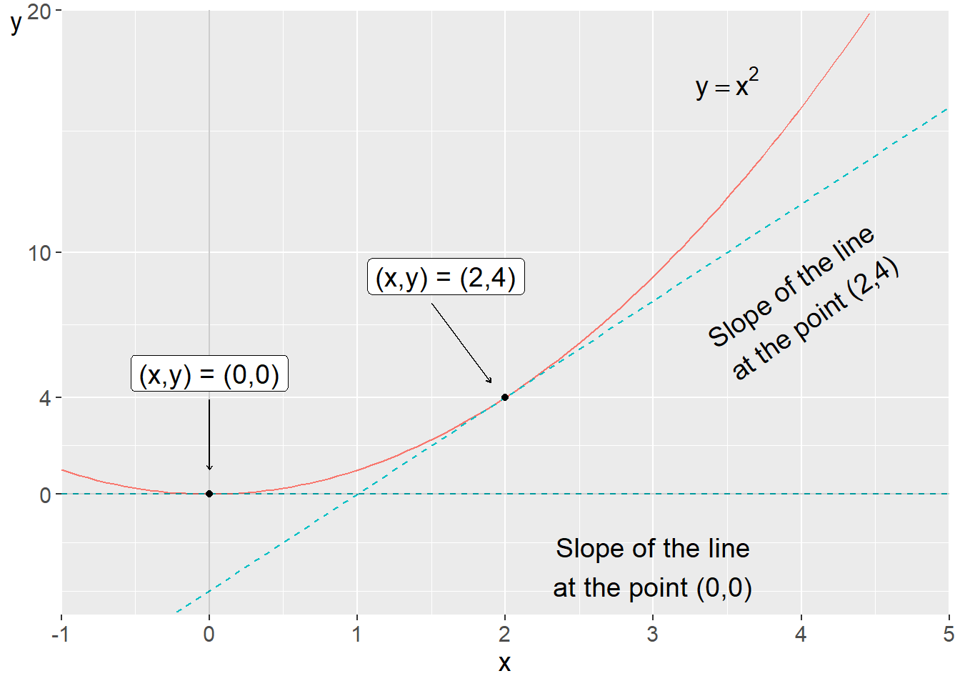
Figure 10.2: The function \(y=x^{2}\)
The derivative indicates the limit of the line’s slope. The limit here refers to how much the function \(f\left(x\right)\) changes at a small change in \(x\). This is described by the derivative’s \(h\)-definition, where the letter \(h\) describes the distance between two values in the variable \(x\)
\[ \begin{equation} f'\left(x\right)=\lim_{h\rightarrow0}\frac{f\left(x+h\right)-f\left(x\right)}{h} \tag{10.2} \end{equation} \]
Equation (10.2) can be read as the derivative of function \(f\left(x\right)\), which we write as \(f'\left(x\right)\), is given by the function value at point x+h minus the function value at point \(x\), as \(h\) goes toward 0, divided by \(h\). The derivative’s \(h\)-definition therefore describes the limit when the distance between the two points \(x\) and \(x+h\) shrinks toward 0. For function \(f\left(x\right)=x^{2}\) we derive this by substituting this function into equation (10.2) :
\[ \begin{align} f'\left(x\right) & =\lim_{h\rightarrow0}\frac{f\left(x+h\right)-f\left(x\right)}{h}\\ & =\lim_{h\rightarrow0}\frac{\left(x+h\right)^{2}-x^{2}}{h}\nonumber \\ & =\lim_{h\rightarrow0}\frac{\left(x+h\right)\left(x+h\right)-x^{2}}{h}\nonumber \\ & =\lim_{h\rightarrow0}\frac{h^{2}+2xh+x^{2}-x^{2}}{h}\nonumber \\ & =\lim_{h\rightarrow0}\frac{h^{2}+2xh}{h}\nonumber \end{align} \]
All terms in the numerator and denominator contain \(h\), which we may simplify:
\[ \begin{align} f'\left(x\right) & =\lim_{h\rightarrow0}\frac{h\times\cancel{h}+2x\cancel{h}}{\cancel{h}}=\lim_{h\rightarrow0}h+2x=2x \end{align} \]
Now we have shown that the function \(y=f\left(x\right)=x^{2}\) has the derivative:
\[ \begin{equation} y'=f'\left(x\right)=2x \end{equation} \]
We now have two functions that both use the variable \(x\): on one hand \(f\left(x\right)=x^{2}\) and on the other hand its derivative, \(f'\left(x\right)=2x\). Let us also figure out what slope the line has in figure 10.2 . The derivative of our function is \(f'\left(x\right)=2x\). To get the slope of the line at a specific point, that is how much y changes when x increases by 1, we substitute the value for x at the current point. In the figure, the points at \(x=2\) and \(x=4\) are marked with dashed lines. If we substitute these values for x into the derivative’s function, we get:
\[ \begin{align} f'\left(2\right) & =2*2=4\\ f'\left(4\right) & =2*4=8\nonumber \end{align} \]
which shows how the line for the function \(y=f\left(x\right)=x^{2}\) slopes at these points.
The dashed lines in the figure are straight lines, which we may calculate backwards in the following way. We know that the derivative is \(f'\left(x\right)=2x\) and that at \(x=2\), \(f'\left(2\right)=2*2=4\). The last is the value for \(y\) at this point. To get the dashed straight line’s equation, we therefore substitute the values we know into such an equation. We seek the following function:
\[ \begin{equation} y=a+bx \end{equation} \]
We already know the values for \(y,b\) and \(x\):
\[ \begin{equation} 4=a+4*2 \end{equation} \]
This gives the following value for \(a\):
\[ \begin{equation} a=4-8=-4 \end{equation} \]
The equation for the dashed line at \(x=2\) in figure 10.2 is therefore:
\[ \begin{equation} y=-4+4x \end{equation} \]
The above walkthrough was relatively elaborate. Fortunately, there are several calculation rules that we may use to avoid doing this process every time we need to use derivatives (see section 10.9 below). The calculation rule for the above example can be formulated as if we have the following function:
\[ \begin{equation} f\left(x\right)=x^{a} \end{equation} \]
its derivative is:
\[ \begin{equation} f'\left(x\right)=ax^{a-1} \end{equation} \]
10.4 The next derivative
For the derived version of \(y=f\left(x\right)\) the following notations say exactly the same thing:
\[ \begin{equation} y'=f'\left(x\right)=\frac{df\left(x\right)}{dx}=\frac{dy}{dx}=\frac{\partial y}{\partial x} \tag{10.3} \end{equation} \]
The symbol \(\partial\) here have the same meaning as the letter \(d\). The expression \(dy/dx\) can be read as a small change of \(y\) divided by a small change of \(x\). This notation is called Leibniz notation, after Wilhelm Leibniz (1646–1716).
So far we have only worked with the first derivative. If we take the derivative of the first derivative, we get the second derivative. This is calculated and written in a similar way as the first derivative. For example:
\[ \begin{align} \text{Function:} & y=f\left(x\right)=x^{3}\\ \text{First derivative: } & \frac{\partial y}{\partial x}=f'\left(x\right)=3x^{2}\nonumber \\ \text{Second derivative } & \frac{\partial}{\partial x}\left(\frac{\partial y}{\partial x}\right)=f''\left(x\right)=2*3x=6x\nonumber \tag{10.4} \end{align} \]
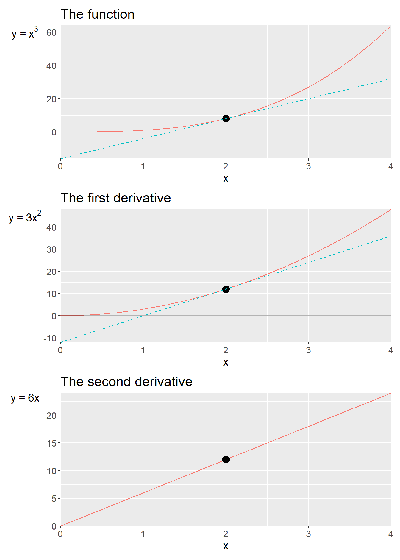
Figure 10.3: The function \(y=f\left(x\right)=x^{3}\) and its first and second derivative
These are three different mathematical expressions: the function, the first derivative and the second derivative. All three expressions are different mathematical functions that use the variable \(x\) as input value, which is evident from the parenthesis with x in the name of each function: \(f\left(x\right),f'\left(x\right)\) and \(f''\left(x\right)\). Figure 10.3 illustrate all these three functions in one graph each, with variable \(y\) on the vertical axis and variable \(x\) on the horizontal axis. In all three graphs, the slope of the line is marked at \(x=2\). Let us calculate the value for each function in equation (10.4) for \(x=2\):
\[ \begin{align} \text{Function: }f\left(2\right) & =2^{3}=8\\ \text{First derivative: }f'\left(2\right) & =3*2^{2}=12\nonumber \\ \text{Second derivative: }f''\left(2\right) & =6*2=12\nonumber \end{align} \]
If we take the derivative of the second derivative, we get what is called the third derivative. The derivative after that is called the fourth derivative and so on. If we start here from the function \(y=f\left(x\right)=x^{3}\), then we have:
\[ \begin{align} y'=f'\left(x\right) & =3x^{2}\\ y''=f''\left(x\right) & =6x\nonumber \\ y'''=f'''\left(x\right) & =6\nonumber \\ y''''=f''''\left(x\right) & =0\nonumber \end{align} \]
where rows 3 and 4 are the third and fourth derivatives of the function \(y=x^{3}\). The fourth derivative is the slope of the slope of the slope of the line’s slope for \(y=x^{3}\), which is 0 for all \(x\). We can see this already in the third derivative, which is defined as \(y'''=6\) for all values of \(x\), which in a graph becomes a horizontal line at \(y=6\).
10.5 Exponent, logarithm and e
We have so far worked with functions where the variable \(x\) stands as the base in a power expression, like \(f\left(x\right)=x^{a}\), where exponent \(a\) is a coefficient (see section 2.8 ). In an exponential function, the variable is instead the exponent. For example:
\[ \begin{equation} y=f\left(x\right)=b^{x} \tag{10.5} \end{equation} \]
where the base \(b\) is a coefficient and the exponent \(x\) is a variable. Sometimes the expression the exponential function is used in definite form, which then refers to \(y=e^{x}\) with the number \(e\) as base. This is sometimes also written as \(y=\exp\left(x\right)=e^{x}\). Let us derive the derivative for the function \(y=b^{x}\) using the derivative’s h-definition (see equation (10.2) ):
\[ \begin{align} y'_{x} & =\lim_{h\rightarrow0}\frac{b^{x+h}-b^{x}}{h}\\ & =\lim_{h\rightarrow0}\frac{b^{x}\left(b^{h}-1\right)}{h}\nonumber \\ & =b^{x}\left(\lim_{h\rightarrow0}\frac{b^{h}-1}{h}\right)\nonumber \tag{10.6} \end{align} \]
In the last step, we factor out \(b^{x}\) since this is independent of \(h\) and therefore is not affected by \(h\) going toward 0. The limit for the expression is dependent on the base \(b\), which is illustrated in figure 10.4 . The solid line shows values for the limit \(\lim_{h\rightarrow0}\left(b^{h}-1\right)/h\) for different \(b\). When \(b=1\), the limit is 0.
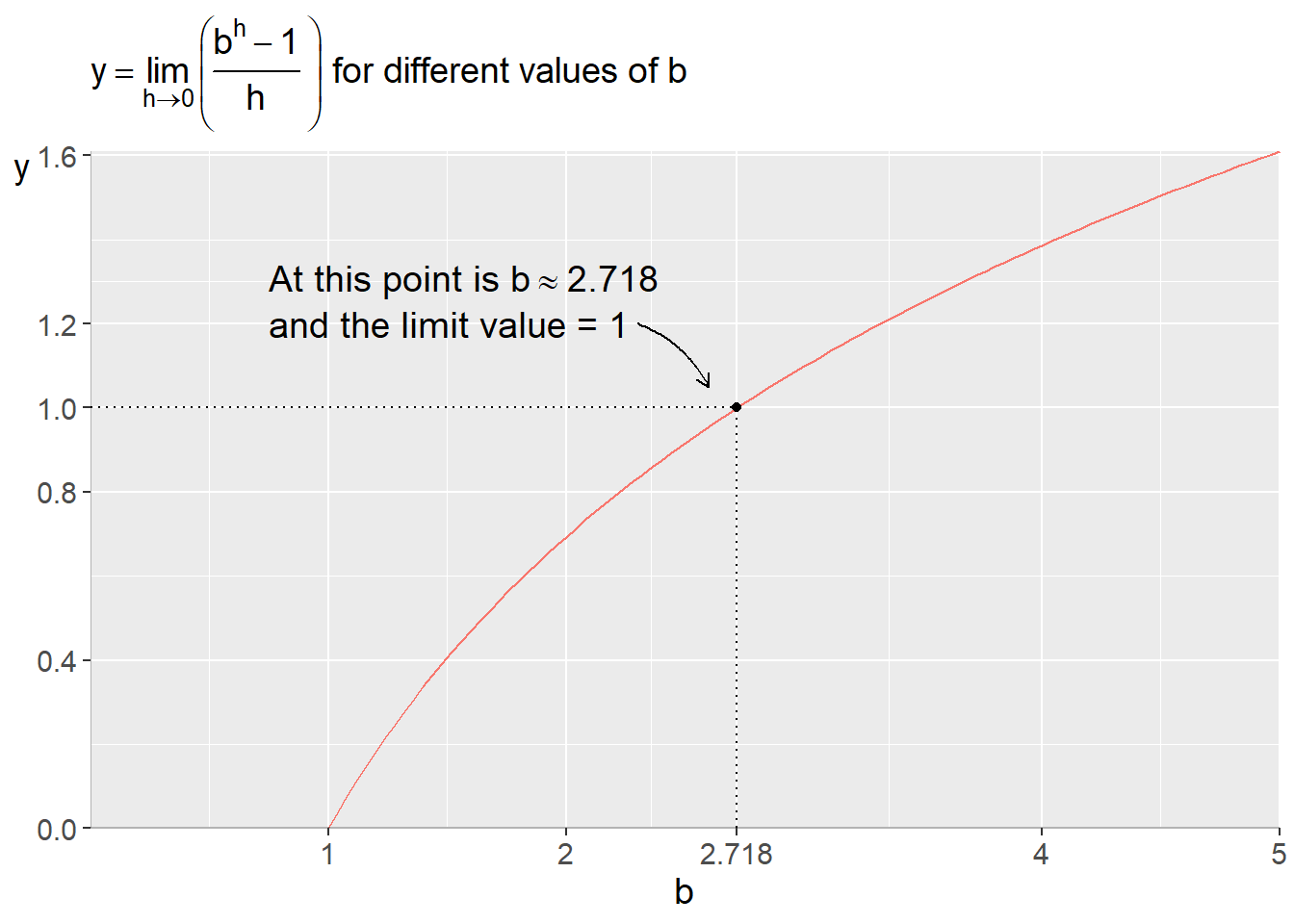
Figure 10.4: The importance of the base \(b\)
The limit \(\lim_{h\rightarrow0}\left(b^{h}-1\right)/h\) from equation (10.6) is equal to 1 when \(b\) is equal to approximately 2.718, which is also marked in figure 10.4 . This number is so commonly occurring that it has received its own name, Euler’s number, and is abbreviated e. We have mentioned this number before. The natural logarithm of the base b in equation (10.6) is the number that \(e\)(approximately 2.718) must be raised to in order to get \(b\). This means that the general result for the equation can be described as the natural logarithm of \(b\). Say now that we have a function with the following form:
\[ \begin{equation} f\left(x\right)=b^{x} \end{equation} \]
Then its derivative
\[ \begin{align} f'_{x}\left(x\right)= & b^{x}\left(\lim_{h\rightarrow0}\frac{b^{h}-1}{h}\right)=b^{x}\log_{e}b=b^{x}\ln b \end{align} \]
If the logarithm’s base \(b\) is equal to the number \(e\), we get:
\[ \begin{align} b^{x}\log_{e}b=e^{x}\ln e=1*e^{x}=e^{x} \tag{10.7} \end{align} \]
This means that if we have a function of the type \(y=f\left(x\right)=e^{x}\), then its derivative is:
\[ \begin{equation} y'_{x}=e^{x} \end{equation} \]
That is, the derivative of function \(y=e^{x}\) is also equal to \(e^{x}\). The second derivative of this function is similarly \(y''_{xx}=e^{x}\). Let us now derive the derivative of the following function:
\[ \begin{equation} y=h\left(x\right)=e^{ax} \end{equation} \]
The variable \(y\) is a function of the variable \(x\) according to the function \(h\left(x\right)\). The letter \(a\) is a constant coefficient and \(e\) is Euler’s number. To calculate the derivative of this function, we again use the derivative’s \(h\)-definition:
\[ \begin{align} y'_{x} & =\lim_{h\rightarrow0}\frac{e^{a\left(x+h\right)}-e^{ax}}{h}=\lim_{h\rightarrow0}\frac{e^{ax}\left(e^{ah}-1\right)}{h}=e^{ax}\left(\lim_{h\rightarrow0}\frac{e^{ah}-1}{h}\right) \tag{10.8} \end{align} \]
In the third step, we factor out \(e^{ax}\) from the parenthesis, which is possible since this factor is not affected by \(h\rightarrow0\). Moving out \(e^{ax}\) thus does not affect the limit. To proceed from here, we may multiply both numerator and denominator in the parenthesis by the constant \(a\), an arbitrary real number. Since \(a\) in the numerator also does not affect the limit, we move this out of the parenthesis. The constant \(a\) in the denominator we leave in place:
\[ \begin{align} y'_{x} & =e^{ax}\left(\lim_{h\rightarrow0}\frac{a}{a}\times\frac{e^{ah}-1}{h}\right)\\ & =ae^{ax}\left(\lim_{h\rightarrow0}\frac{e^{ah}-1}{ah}\right)\nonumber \\ & =ae^{ax}\left(\lim_{h\rightarrow0}\frac{e^{ah}-1}{ah}\right)\nonumber \\ & =ae^{ax}\nonumber \end{align} \]
When we move a out of the parenthesis, both numerator and denominator go toward 0, which is why the limit goes toward 1. In the last line we therefore remove the limit and only have \(y'_{x}=ae^{ax}\) left. This expression has the same form as what we derived in equation (10.7) . We may summarize this as a general calculation rule. If we have a function with the form:
\[ \begin{equation} y=f\left(x\right)=e^{g\left(x\right)} \end{equation} \]
its derivative is:
\[ \begin{equation} y'_{x}=g'_{x}e^{g\left(x\right)} \end{equation} \]
These examples also make it easy to continue with other types of functions, for example the following power function:
\[ \begin{equation} y=f\left(x\right)=b^{ax} \tag{10.9} \end{equation} \]
where the letters b and a are coefficients and \(y\) and \(x\) are variables. One way to derive the derivative of equation (10.9) is to rewrite the expression as a power with base \(e\), Euler’s number:
\[ \begin{equation} y=f\left(x\right)=b^{ax}=e^{\ln b^{ax}}=e^{ax\ln b} \end{equation} \]
We here take the natural logarithm of our function \(b^{ax}\), which gives \(\ln b^{ax}=ax\ln b\). We use this as an exponent to the base \(e\), which gives us an expression that we can differentiate:
\[ \begin{align} f'_{x}\left(x\right) & =\left(a\ln b\right)e^{ax\ln b}=\left(a\ln b\right)b^{ax} \end{align} \]
10.6 The derivative of \(\boldsymbol{\log x}\)
Let us now differentiate the following function:
\[ \begin{equation} y=\log x \end{equation} \]
where \(\log x\) is the logarithm of \(x\) with arbitrary base \(b\), where \(b>0\) and \(b\neq1\). We use the derivative’s \(h\)-definition:
\[ \begin{align} y'=\left(\log x\right)' & =\lim_{h\rightarrow0}\frac{\log\left(x+h\right)-\log\left(x\right)}{h} \end{align} \]
Since \(\log a-\log b=\log\left(a/b\right)\) we write:
\[ \begin{equation} y'=\lim_{h\rightarrow0}\frac{\log\left(1+\frac{h}{x}\right)}{h} \end{equation} \]
We factor out the numerator \(h^{-1}\):
\[ \begin{equation} y'=\lim_{h\rightarrow0}\frac{1}{h}\log\left(1+\frac{h}{x}\right) \end{equation} \]
Let us now define \(z=h/x\) so \(1/h=\frac{1}{z}\frac{1}{x}\):
\[ \begin{equation} y'=\lim_{h\rightarrow0}\frac{1}{x}\frac{1}{z}\log\left(1+z\right) \end{equation} \]
Note that as \(h\rightarrow0\), \(z\rightarrow0\) as well. The multiplier \(1/z\) in front of the logarithm we move up to the exponent:
\[ \begin{equation} y'=\frac{1}{x}\lim_{h\rightarrow0}\log\left(1+z\right)^{1/z} \tag{10.10} \end{equation} \]
We shall now look more closely at the part of the expression that consists of \(\left(1+z\right)^{1/z}\). Let us temporarily rewrite this to the following function:
\[ \begin{equation} y=\left(1+z\right)^{1/z} \end{equation} \]
and look at some values in a graph. Figure 10.5 shows the line for this function over some values for \(z\) between \(-1\) and 2. Due to the exponent, this function is not defined for \(z=0\).
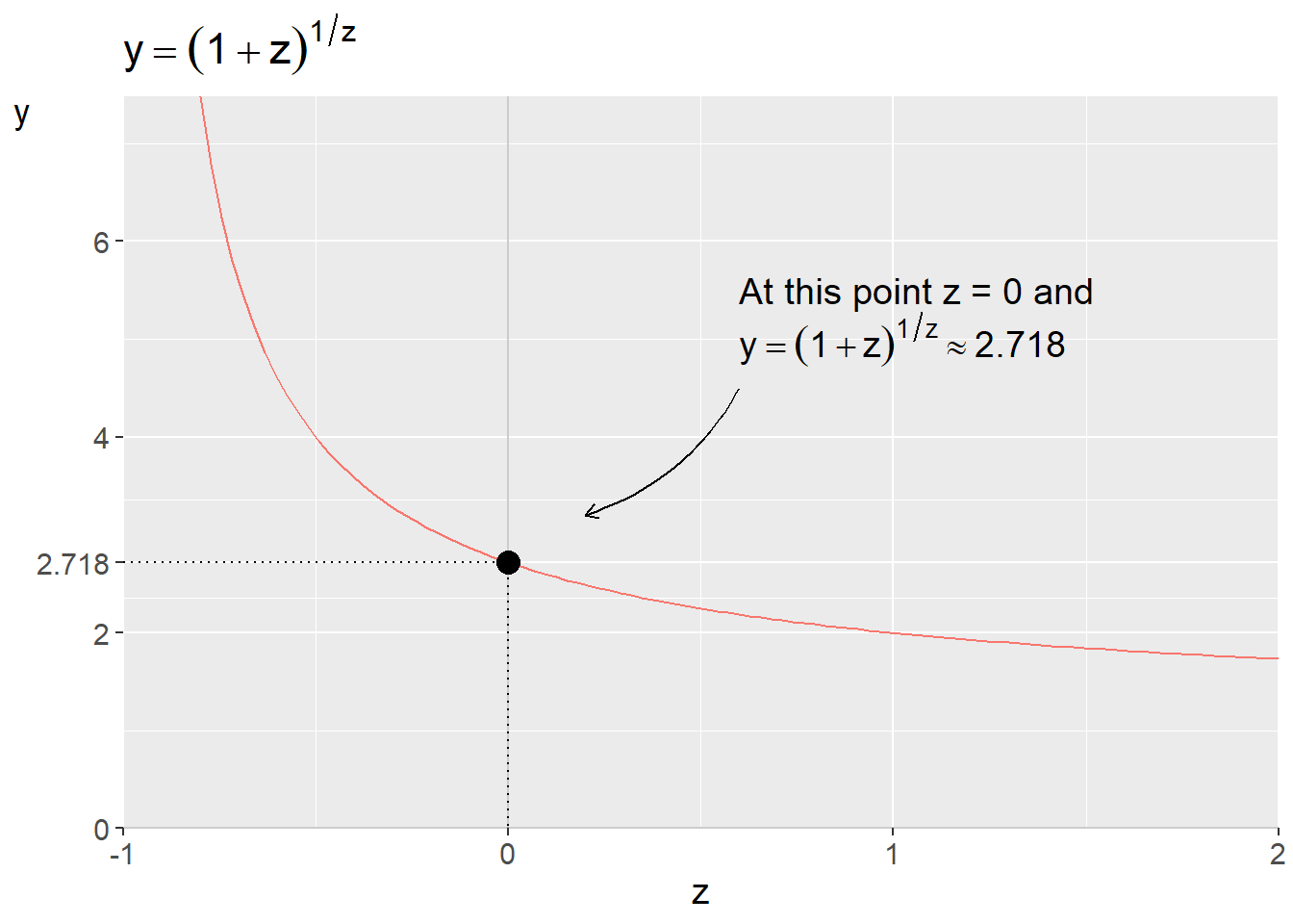
Figure 10.5: The function \(y=\left(1+z\right)^{1/z}\)
Note how the limit for this function approaches the value 2.718 as z approaches 0. The number 2.718 we recognize already as Euler’s number, \(e\). The limit for the expression in equation (10.10) is equal to \(e\):
\[ \begin{align} y' & =\frac{1}{x}\left(\lim_{z\rightarrow0}\log\left(1+z\right)^{1/z}\right)=\frac{1}{x}\log e \end{align} \]
As mentioned at the beginning of the example, the logarithm here has base b. Let us now change base to e, so that we get the natural logarithm. We went through this in section 5.5 where in equation (5.5) we had the general rule for changing base between logarithms:
\[ \begin{equation} \log_{a}x=\frac{\log_{b}x}{\log_{b}a} \end{equation} \]
In this case this means:
\[ \begin{equation} \log_{b}e=\frac{\ln e}{\ln b}=\frac{1}{\ln b} \end{equation} \]
The derivative of \(\log x\) then becomes:
\[ \begin{equation} y'_{x}\left(x\right)=\left(\log_{b}x\right)'_{x}=\frac{1}{x\ln b} \tag{10.11} \end{equation} \]
When we have base \(b=e\) the derivative is:
\[ \begin{equation} y'_{x}=\left(\ln x\right)'_{x}=\frac{1}{x} \tag{10.12} \end{equation} \]
10.7 L’Hôpital’s rule
Here follows a simplified description of L’Hôpital’s rule (also called Bernoulli’s rule), which is a useful calculation rule for derivatives. Suppose we have the functions \(f\left(x\right)\) and \(g\left(x\right)\) and these go toward 0 when \(x\) goes toward the limit \(a\). Alternatively that the function \(g\) approaches infinity. We calculate a constant derivative sufficiently close to the limit \(a\), in such a way that we get the following:
\[ \begin{equation} \lim_{x\rightarrow a}\frac{f'}{g'} \end{equation} \]
For these functions the following then applies:
\[ \begin{equation} \lim_{x\rightarrow a}\frac{f\left(x\right)}{g\left(x\right)}=\lim_{x\rightarrow a}\frac{f'_{x}\left(x\right)}{g'_{x}\left(x\right)} \tag{10.13} \end{equation} \]
This is called L’Hôpital’s rule and means that the limit for function \(f\) divided by function \(g\) as \(x\) goes toward \(a\) is the same as the limit for the derivative of \(f\) divided by the derivative of \(g\) as \(x\) goes toward \(a\). We illustrate the usefulness of L’Hôpital’s rule with the function:
\[ \begin{equation} y=k\left(x\right)=\frac{x^{2}+3}{x-2} \end{equation} \]
Function \(k\left(x\right)\) is not defined for \(x=2\), since the denominator then becomes 0. To facilitate the calculation of the limit for \(x=2\), we then use L’Hôpital’s rule. We define the numerator as \(f\left(x\right)=x^{2}+3\) and the denominator as \(g\left(x\right)=x-2\). We have the derivatives \(f'_{x}=2x\) and \(g'_{x}=1\). Now we calculate the limit as \(x\rightarrow2\):
\[ \begin{equation} \lim_{x\rightarrow2}k\left(x\right)=\lim_{x\rightarrow2}\frac{2x}{1}=4 \end{equation} \]
The number 4 comes from \(x\rightarrow2\) and \(2x=2*2=4\). The limit for the derivative of \(k\left(x\right)\) with respect to \(x\) as \(x\rightarrow2\) is thus 4. According to L’Hôpital’s rule, this is also the limit for the quotient \(\frac{f\left(x\right)}{g\left(x\right)}\) as \(x\rightarrow2\).
10.8 Partial derivative
When we took the derivative of \(f\left(x\right)\) above, we wrote \(f'\left(x\right)\) and since we only have one variable in the function, we understand that this refers to taking the derivative with respect to the variable \(x\). We may also write to our variable to be extra clear:
\[ \begin{equation} f'_{x}\left(x\right)=\text{the derivative of f with respect to variable x} \end{equation} \]
If we have several variables, such as \(f\left(x,y\right)\), we may calculate the derivative for each variable. This is called the partial derivative. For the derivative of function \(f\) with respect to \(x\) and \(y\) respectively, we write \(f'_{x}\) and \(f'_{y}\). If we differentiate \(f\) with respect to one variable \(x\) we do not differentiate with respect to other variables in the same function. Other terms in the function are treated as constants. Take the following function:
\[ \begin{align} f\left(x,y\right) & =x^{2}+y^{2} \end{align} \]
We shall differentiate this with respect to \(x\) and \(y\), and thereafter differentiate the results with respect to \(x\) and \(y\) again:
\[ \begin{align} f'_{x} & =2x\\ f'_{y} & =2y\nonumber \\ f''_{xx} & =2\nonumber \\ f''_{yy} & =2\nonumber \end{align} \]
We may also differentiate \(f\) first with respect to first \(x\) and get \(f'_{x}=2x\), and then differentiate this function with respect to \(y\):
\[ \begin{equation} f''_{xy}=0 \end{equation} \]
The same thing if we instead differentiate \(f\) first with respect to \(y\) and then \(x\):
\[ \begin{equation} f''_{yx}=0 \end{equation} \]
Let us take another example with the following function:
\[ \begin{align} g\left(x,y\right) & =x^{2}y^{2} \end{align} \]
The first and second derivatives of function \(g\) with respect to \(x\) and \(y\):
\[ \begin{align} g'_{x} & =2xy^{2}\\ g''_{xx} & =2y^{2}\nonumber \\ g'_{y} & =2yx^{2}\nonumber \\ g''_{yy} & =2x^{2}\nonumber \\ g''_{xy} & =4xy\nonumber \\ g''_{yx} & =4yx\nonumber \end{align} \]
10.9 Differentiation rules
Table 10.1 describes with general equations some examples of rules for differentiation, where \(x\) is the variable and the letters \(a\), \(b\) and \(c\) are constants. The letter \(e\) is Euler’s number. \(f\left(x\right)\) refers to function \(f\) of \(x\) and \(f'_{x}\) refers to the first derivative of this function, with respect to \(x\).
| Function | First derivative | |
|---|---|---|
| 1 | \(f\left(x\right)=bx^{a}+c\) | \(f'_{x}\left(x\right)=abx^{a-1}\) |
| 2 | \(f\left(x\right)=\frac{1}{x}=x^{-1}\) | \(f'_{x}\left(x\right)=-1\cdot x^{-2}=-1/x^{2}\) |
| 3 | \(f\left(x\right)=\sqrt{x}=x^{\frac{1}{2}}\) | \(f'_{x}\left(x\right)=\frac{1}{2}x^{-\frac{1}{2}}=1/\left(2\sqrt{x}\right)\) |
| 4 | \(\frac{1}{f\left(x\right)}=\left(f\left(x\right)\right)^{-1}\) | \(\left(\frac{1}{f\left(x\right)}\right)'_{x}=-\frac{f'_{x}\left(x\right)}{\left[f\left(x\right)\right]^{2}}\) |
| 5 | \(f\left(x\right)=b^{ax}\) | \(f'_{x}\left(x\right)=\left(a\ln b\right)b^{ax}\) |
| 6 | \(f\left(x\right)=e^{g\left(x\right)}\) | \(f'_{x}\left(x\right)=g'_{x}e^{g\left(x\right)}\) |
| 7 | \(f\left(x\right)=e^{ax}\) | \(f'_{x}\left(x\right)=ae^{ax}\) |
| 8 | \(f\left(x\right)=\log x\), \(g\left(x\right)=\ln x\) | \(f'_{x}\left(x\right)=\frac{1}{x\ln b}\), där \(b\) är log bas., \(g'_{x}\left(x\right)=\frac{1}{x}\) |
| Combination | First derivative | |
|---|---|---|
| 1 | \(\left(f+g\right)\left(x\right)=f\left(x\right)+g\left(x\right)\) | \(\left(f+g\right)'_{x}=f'_{x}+g'_{x}\) |
| 2 | \(\left(f-g\right)\left(x\right)=f\left(x\right)-g\left(x\right)\) | \(\left(f-g\right)'_{x}=f'_{x}-g'_{x}\) |
| 3 | \(\left(f\times g\right)\left(x\right)=f\left(x\right)\times g\left(x\right)\) | \(\left(f\times g\right)'_{x}=f'_{x}\left(x\right)g\left(x\right)+f\left(x\right)g'_{x}\left(x\right)\) |
| 4 | \(\left(f/g\right)\left(x\right)=\frac{f\left(x\right)}{g\left(x\right)}\) | \(\left(\frac{f}{g}\right)'_{x}=\frac{f'_{x}\left(x\right)g\left(x\right)+f\left(x\right)g'_{x}\left(x\right)}{\left[g\left(x\right)\right]^{2}}\) |
| 5 | \(f\circ g=f\left(g\left(x\right)\right)\) | \(f'_{x}\left(g\left(x\right)\right)g'_{x}\left(x\right)\) |
In section 4.9 we went through how we may use addition, subtraction, multiplication and division on functions, like \(\left(f+g\right)\left(x\right)=f\left(x\right)+g\left(x\right)\). In the same section we introduced composite functions, such as \(y=f\left(g\left(x\right)\right)\). Table 10.2 summarizes calculation rules for derivatives where two functions are added (row 1), subtracted (row 2), multiplied (row 3), divided (row 4) or composed (row 5). We illustrate these calculation rules with the functions:
\[ \begin{align} f\left(x\right) & =x^{2}\\ g\left(x\right) & =3-2x\nonumber \end{align} \]
The first derivative of each function with respect to \(x\) is:
\[ \begin{align} f'_{x}\left(x\right) & =2x\\ g'_{x}\left(x\right) & =-2\nonumber \end{align} \]
If the functions are added, we get:
\[ \begin{align} f+g & =x^{2}+3-2x\\ \left(f+g\right)'_{x}=f'+g' & =2x-2\nonumber \end{align} \]
With subtraction:
\[ \begin{align} f-g & =x^{2}-3+2x\\ \left(f-g\right)'_{x}=f'-g' & =2x+2\nonumber \end{align} \]
Row three in table 10.2 describes what is called the product rule:
\[ \begin{align} f\times g & =x^{2}\left(3-2x\right)\\ \left(f\times g\right)'_{x}=f'g+fg' & =2x\left(3-2x\right)-2x^{2}\nonumber \end{align} \]
Row four in table 10.2 describes the quotient rule. This shows how to calculate the derivative when one function is divided by another function:
\[ \begin{align} \frac{f}{g} & =\frac{x^{2}}{3-2x}\\ \left(\frac{f}{g}\right)'_{x}=\frac{f'g+fg'}{g^{2}} & =\frac{2x\left(3-2x\right)-2x^{2}}{\left(3-2x\right)^{2}}\nonumber \end{align} \]
Row five in table 10.2 describes the chain rule, which shows how to calculate the derivative for composite functions. For example:
\[ \begin{align} f\left(g\left(x\right)\right) & =\left(3-2x\right)^{2} \end{align} \]
We also have that \(g'_{x}=-2\) and \(f'_{g\left(x\right)}=2\left(3-2x\right)\). The derivative of \(f\left(g\left(x\right)\right)\) with respect to \(x\) is then:
\[ \begin{align} f\left(g\left(x\right)\right)'_{x} & =f'_{g}\left(g\right)g'_{x}=2\left(3-2x\right)\left(-2\right)=-4\left(3-2x\right) \end{align} \]
10.10 Elasticity
A measure that is often used in social science is elasticity. This indicates how much one variable changes in percentage terms at a percentage change in another variable. Say for example that \(q\) is the number of sold units of this good (the market’s demand), and \(p\) is the price for this good.
Change between two price levels can be written as \(\Delta p=p_{2}-p_{1}\), which we read as the difference between price level 1 and price level 2. The letter \(\Delta\)(the Greek letter capital delta) symbolizes change here. Change between two quantities: \(\Delta q=q_{2}-q_{1}\). The price elasticity can then be defined as:
\[ \begin{equation} \text{price elasticity: }\frac{\frac{\Delta q}{q}}{\frac{\Delta p}{p}}=\frac{\frac{q_{2}-q_{1}}{q_{1}}}{\frac{p_{2}-p_{1}}{p_{1}}} \end{equation} \]
This is percentage change of \(q\) divided by percentage change of \(p\). If demand \(q\) changes a lot when \(p\) changes, this means that the good has high price elasticity, customers are very price-sensitive. If demand \(q\) barely changes at all when \(p\) changes, price elasticity is low and customers are relatively price-insensitive.
In equation (10.3) we described the derivative using the letter \(d\) and the symbol \(\partial\). The derivative gives us the slope of the line at a specific point. Similarly, we may compare the elasticity at a specific point, which is called point elasticity. Say for example that a large store sells milk for 10 USD per package. Every week 100 packages are sold. In January, the store decides to raise the price by 20%, to 12 USD per package. In the long run, sales drop to 97 packages per week. The price elasticity of demand for milk is then:
\[ \begin{align} \frac{\partial q/q}{\partial p/p} & =\frac{-0.03}{0.2}=-0.15 \end{align} \]
When the price increases by 20%, demand decreases by 3%, which is why the price elasticity is \(-0.15\%\). We do not know if this elasticity applies to all price levels. Studying price elasticity in reality is more complex than this example, see chapter 27 .
10.11 Chapter summary
The limit, limes, for a function describes the value the function approaches when it comes infinitely close to a point. Example: \(\lim_{x\rightarrow0}\frac{1}{x}=\infty\) and \(\lim_{x\rightarrow\infty}\frac{1}{x}=0\).
The derivative is a function that describes the limit for a line’s slope at a point. The derivative’s \(h\)-definition: \(f'\left(x\right)=\lim_{h\rightarrow0}\frac{f\left(x+h\right)-f\left(x\right)}{h}\), where h indicates the distance between two values in the variable \(x\).
For the function \(f\left(x\right)\) we may write the first derivative with respect to \(x\) as \(f'_{x}\), the second derivative as \(f''_{xx}\) and the third derivative as \(f'''_{xxx}\). Example: \(y=f\left(x\right)=x^{3}\), \(f'_{x}=3x^{2}\), \(f''_{xx}=6x\) and \(f'''_{xxx}=6\).
The function \(y=f\left(x\right)=a+bx\) has the slope \(b\) for all values of \(x\) that the function is defined for. The derivative can be written \(f'=b\).
Partial derivative: differentiate a function with several variables with respect to one variable at a time. Example: \(y=f\left(x,z\right)=x^{2}+z^{2}\) has first derivative \(f'_{x}=2x\) and \(f'_{z}=2z\).
Examples of differentiation rules:
-\(f\left(x\right)=bx^{a}+c\) gives \(f'_{x}=abx^{a-1}\).
-\(g\left(x\right)=b^{ax}\) gives \(g'_{x}\left(x\right)=\left(a\ln b\right)b^{ax}\).
-\(h\left(x\right)=\log x\) gives \(h'_{x}\left(x\right)=1/\left(x\ln b\right)\).
• Examples of differentiation with combined and composite functions
-\(\left(f+g\right)\left(x\right)'_{x}=f'_{x}+g'_{x}\)
-\(\left(f-g\right)\left(x\right)'_{x}=f'_{x}-g'_{x}\)
-\(\left(\frac{1}{f\left(x\right)}\right)'_{x}\)= \(\left(f\left(x\right)^{-1}\right)'_{x}\) \(=-f'_{x}f^{-2}=\frac{-f'_{x}}{\left(f\left(x\right)\right)^{-2}}\)
Product rule: \(\left(f\left(x\right)g\left(x\right)\right)'_{x}=\left(\left(f\times g\right)\left(x\right)\right)'_{x}=f'g+g'f\)
Quotient rule: \(\left(\frac{f\left(x\right)}{g\left(x\right)}\right)'_{x}=\frac{f'_{x}g+fg'_{x}}{g}\)
Chain rule: \(f\left(g\left(x\right)\right)'_{x}=g'f'\).
L’Hôpital’s rule: \(\lim_{x\rightarrow a}\frac{f\left(x\right)}{g\left(x\right)}=\lim_{x\rightarrow a}\frac{f'_{x}\left(x\right)}{g'_{x}\left(x\right)}\).